.png)
In many ways, spreadsheets are one of the greatest tools available to STEM consumers at any level of learning. Each of the four included fields, from Science to Mathematics, can benefit from their unique ability to serve as a calculator, data organizer, and graphing tool all at once. Not only that, but their inclusion in free-to-use suites such as the basic plan of Google Workspace make them more accessible than any other piece of mathematical software. Despite their ease of access, spreadsheets still fall under the radar for many STEM enjoyers. Why? There are many reasons, but the most obvious is that they can be tricky to use for those unaccustomed to their features and quirks. In this slightly unorthodox article, I will be walking you through some of the basic features of spreadsheets and giving you a hands-on introduction to one of the many ways they are used in the STEM world today: population simulation.
Population simulation is the art of using mathematical processes to take some basic data from a population and extrapolate it into a theoretical future. This process can be hugely useful in many fields, but it is especially useful to biologists and other scientists who research populations of living creatures. Using tools like spreadsheets, we can predict how a population of organisms will develop over time based on only a generation or two's worth of data. These "educated guesses" can help us shape how we interact with populations in the future, and we can use them as something to test reality against as time passes. Even if a model proves incorrect, researchers will have a better clue as to what is and isn't interfering with that population's development, allowing them to move forward with a better understanding of the population they are observing.
In today's guided activity, you will assume the role of a biologist and simulate how allele frequencies change within a population. Along the way, you will be introduced to some of the most useful features of spreadsheets, which will open up your horizons and prepare you to try out any spreadsheet ideas that pop into your head as you investigate other STEM topics in the future.
Hold Up...Allele Frequencies?
Before we get started with the spreadsheet, it's important to clear the air about the biological concepts we'll be using as the theme for our exploration. If you feel comfortable with concepts of Mendelian Genetics, feel free to skip onto the next section. If not, here's a quick overview:
Mendelian Genetics are a genre of genetics named after the German scientist Gregor Mendel, who came up with the concept of alleles when researching the inheritance of flower color in pea plants. Through his research and subsequent expansions on it, it has been demonstrated that variations of a given trait, such as the flower color in a plant, are the result of packets of genetic information called alleles. The number of alleles per trait can vary, but Mendel's experiments and the demonstration in this article will revolve around a trait that has only two alleles. Each trait in an offspring takes half of its alleles from one parent and half of its alleles from the other parent, and the combination of alleles present determines how the trait will be expressed. Alleles are typically represented by letters. Using Mendel's research as an example, the allele for purple flowers might be called "P" while the allele for white pea flowers might be called "p." For the ease of spreadsheet use in this experiment, we will use different letters for different alleles; instead of being "p," the white flower allele might be called "W" in this experiment.
Different alleles can interact with one another in many different ways to produce traits. In general, however, one allele is dominant while the other allele is recessive. Dominant alleles will cause their trait to be expressed if they are present at all in an organism's genotype, which is the combination of alleles it has for a certain trait. For example, if the "P" allele is dominant in a certain species of plant, organisms that have the genotype "PW" (one purple allele and one white allele) will have purple flowers even though a white allele is present. Recessive alleles, on the other hand, will only express their trait if they are the only allele present in an organism's genotype. If we consider the "W" allele in those plants to be a recessive allele, then a plant would only have white flowers if its genotype was "WW." Dominance isn't always black-and-white in nature, however. One allele may have incomplete dominance over another allele, causing their two traits to blend together. Going back to the flower example, if the "P" allele was incompletely dominant over the "W" allele, plants with the "PW" genotype might have pale purple flowers instead of purely purple or purely white flowers. We will use principles of incomplete dominance as a part of this experiment. It is also possible for two alleles to be codominant, meaning that they have equal "power" to one another and express equally together. A plant with the "PW" genotype where both alleles were codominant to one another might have purple flowers with white splotches.
Different traits--and, by extension, different alleles--may help some organisms be more successful than other members of their species in their shared environment. According to principles of natural selection, those organisms with more beneficial traits are more likely to survive and pass their traits (alleles) down to their offspring. Changes in a population's allele frequency help reflect which traits and alleles are most successful. The more frequently a trait (allele combination) shows up in a population, the more beneficial it tends to be. Allele frequency is calculated as follows: number of copies of an allele divided by the total number of alleles present in the population. The frequencies of all alleles in a population must add up to exactly 1; if the "P" allele appears 80% of the time (a frequency of 0.8), the other allele for the trait, the "W" allele, must appear 20% of the time (a frequency of 0.2).
Other Terms that Will Appear in this Experiment:
Gametes: The two sex cells, one from each parent, that fuse to produce an offspring. If a given trait has two allele slots, each gamete will contain one allele for that trait.
Zygote: A living offspring produced by the fusion of two gametes.
Phenotype: An organism's physical traits/appearance, which reflects the interaction of the alleles present in its genotype. A "PW" plant (where the purple "P" allele is dominant over the white "W" allele) would have a purple phenotype, even though a white allele is present in its genotype.
Getting Started With Spreadsheets
Now that we've familiarized ourselves with the biological principles we'll be using in this demonstration, it's time to get started on the spreadsheets themselves. Most common spreadsheet softwares, from Google Sheets to Microsoft Excel, operate using the same formulas. Regardless of which program you use, you should be able to replicate this experiment with little issue. Since Microsoft Excel requires a Microsoft Office subscription, however, this tutorial will focus specifically on the free-to-use alternative from Google, Google Sheets. If you don't know how to translate differences in menu format from Google Sheets to other programs, it is recommended that you follow along in Google Sheets for your first attempt at spreadsheet building. As long as you have a Google Account, you should be able to access this useful software for free!
Opening up the Google Sheets app, you will see a menu like this:

This is the template selection menu. Google Sheets offers many pre-made templates for data organization, calculation, and more, but, for the purposes of this tutorial, you should start with the "Blank" template that should be on the far left.
When it opens up, you should see a wide open spreadsheet, ready to be customized:

Before we continue on, it's important to point out a few of the features that will be referenced throughout the rest of this exploration. Each little box on the spreadsheet is called a cell. Each cell has a specific "name" within the spreadsheet that is a combination of the letter at the top of its column (vertical line of cells) and the number at the left side of its row (horizontal line of cells). The cell highlighted blue in the above image is known as cell A1, because it is the first cell in the A column.
At the bottom of the spreadsheet is a bar for all of the individual pages, or sheets, in the spreadsheet. Each sheet is essentially a whole new blank document. New sheets can be added to the spreadsheet by clicking on the plus button on the far left side of the bottom bar. Sheets that already exist can also be duplicated by right-clicking the sheet tab you want to duplicate and selecting "Duplicate" from the menu that pops up. This will come in handy later.
Starting the Simulation
With the basics out of the way, we can finally get started with our experiment. Before we set up anything else about our population simulation, we must start by doing two things: defining our alleles and defining our allele frequencies.
Let's say we're looking at an organism with a trait that is very related to its survival. This trait has two alleles, allele "A" and allele "B."
Tip! Put Names to Faces.
It's fine enough to think of this as a simulation about some unspecified organism, with some unspecified trait, but it's even more engaging to come up with a species to theme your population experiment around. Maybe you're simulating a population of unicorns, and alleles "A" and "B" affect the horn size of each individual. Or, maybe, if you're more the realistic type, you can pretend that you're researching your favorite real-life species. The possibilities are endless, and moving the concepts involved into less abstract territory can really help you connect with what you're doing. It's also great for helping you take this experiment to new heights after the tutorial is concluded; if you know what "population" you are researching and what purpose each "trait" serves, you can tweak the settings in a realistic way to try out new things--like a real biologist would.
To demonstrate the results quicker, let's say these alleles have incomplete dominance, so individuals with the genotype "AB" will have a fusion of the "A" and "B" traits. The technical reasons why this distinction is important will become clear later on; for now, let's focus on the individual alleles themselves.
What about the scientific reasons?
Incomplete dominance prevents a dominant allele from "masking" a recessive allele. If the recessive allele is less successful from a survival standpoint, it may still survive in a population by "piggybacking" off the more successful dominant allele. The effects of natural selection take much longer to become noticeable if this is the case, even in a simulation. To see the best and most dramatic results, incomplete dominance allows the frequency of the less successful allele to be impacted by natural selection, even if it is paired with a more successful allele.
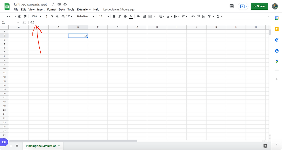
How frequently does allele "A" appear in the population? What about allele "B"? In this experiment, it's up to you! Let's start with allele "A." In cell D2 of your spreadsheet, put down a decimal number between 0 and 1. If you want to start out simple, go with a number rounded to the nearest tenth--like 0.8, 0.5, or 0.2. You can type directly into the box itself, or you can type it into the formula bar, which is a useful (but rather subtle) part of the spreadsheet that will be crucial for instructing it to make calculations for us later on. The formula bar is located here:
Now that you've determined the frequency of allele "A," it's a good idea to create a label for it so that you (and any others who read your spreadsheet) will be able to know what that cell references. Type a quick label, like "Frequency A =" in cell C2.
Now, we need to write down the frequency of allele "B," which should be equal to one minus the frequency of allele "A." It's simple enough to do that math in your head, but it's even simpler to make the spreadsheet do the math for you! Click on cell D3. Then, copy the following into the formula bar (without the quotation marks): " =1-D2 " and click return/enter on your keyboard. Instead of what you just typed, the correct value will appear in cell D3! You have just created your very first formula. Let me break down how it works:
By typing an equals sign, you "prime" the spreadsheet to look for a formula. This can be as simple as a calculator prompt, like what you used to calculate the frequency of allele "B," or more complicated, as you will see later on.
The spreadsheet then reads everything after the equals sign like a graphing calculator would, with the added benefit of being able to reference the values found in cells. Instead of needing to type the frequency of allele "A," all you had to type was "D2" to tell the spreadsheet to look for the value found in cell D2. This allows you to perform much more complicated operations AND tell the spreadsheet to calculate something new without tweaking the formula in the slightest. Don't believe me? Put a different decimal value in cell D2. The value in cell D3 will change automatically as soon as you click "enter."
Add a label for the frequency of allele "B" in cell C3. Your spreadsheet should now look like this:
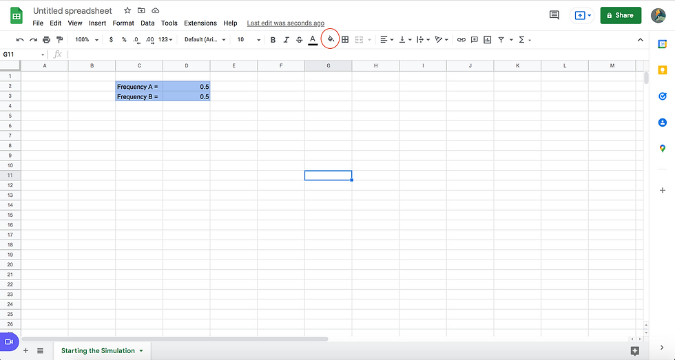
Well, not quite. You may notice that my reference cells are now colored blue. I did this to draw the eye to these important values and help keep myself from accidentally highlighting cells that don't need to be altered later on. If you'd like to do the same, all you need to do is click the paint bucket icon (circled in red above) and select a color of your choice with which to highlight the cells. Just make sure that the color isn't too intense, or it may be hard to read the text you've put there later on.
Laying the Groundwork
With the allele frequencies determined, you are now ready to move on to the bulk of the simulation. This is where most of the hard work happens; you will build increasingly complex formulas and set your sheet up to simulate a single generation of your population. Once this step is complete, you will be able to sit back and watch the magic happen without typing more than a single value for each new generation!
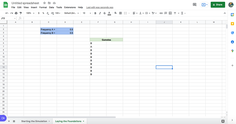
We'll start off small with some labeling work. We are about to set up two columns of "gametes," which will contain randomly generated alleles. These two columns only need one label, so, instead of typing the same word at the top of both columns, you can merge the two cells at the top to create a single label. Highlight cells F5 and G5 by left clicking on one and dragging your cursor over to the other. Then, click on the Format menu and select "Merge Cells" from the dropdown. In the next menu that opens, pick "Merge All" to combine the two cells together into one. Now, when you type "Gametes" into the merged cell, you can center the text so that it hovers over both columns! Merging can be very useful from a graphical standpoint, so, while not essential to this experiment, it's a nice trick to have on hand if you want to create more visual intrigue or distinction in any future spreadsheets.

Now, we will work to compose a formula that randomly generates alleles for us. Spreadsheets actually have some great built-in formulas that help you generate random numbers without having to roll them each by hand. In order to get a random number from 0 to 1, all you need to do is type the following formula into the formula bar of any cell:
=rand()
This is a named formula, or a formula that can be referenced in the spreadsheet by a name rather than a series of mathematical instructions like plus or minus symbols. There are dozens of named formula on offer, but the =rand() function is the one that allows us to easily generate a number from 0 to 1. Try typing it into cell F6; you'll see that, when you press enter, a lengthy and entirely random decimal number awaits you.

Any time you edit the spreadsheet, the random number will be re-rolled, allowing you to quickly generate a whole slew of random numbers in a handful of seconds.
By itself, this formula isn't very useful to our cause. We can compare it to our allele frequencies and manually select the appropriate allele, but such a thing would be needlessly time-consuming. Using another named formula, it is possible to make the spreadsheet do the comparisons for you! Enter, the "=IF" formula.
The "=IF" formula allows you to compare two things and produce different outcomes based on how those two things compare. We want to compare a random value to the frequency (probability) of our first allele, allele "A." If that random value is less than or equal to the frequency of allele "A," we want "A" to appear in the cell. If that random value is greater than the frequency of allele "B," we want "B" to appear instead. Have a look at the syntax, or structure, of the formula and see if you can figure out the complete formula:
=IF(value 1<=value 2,"a specific value that appears if the inequality is true","a specific value that appears if the inequality is false")
Less than or equal to
You may notice the "<=" between value one and value two in the above formula. This is how we tell the spreadsheet we want to see if the first value is less than or equal to the second value. If you just wanted to see if the first value is less than the second value, you could replace that with "<" instead. The same would go for greater than (">"), greater than or equal to (">="), or equal to ("=").
If you came up with something along the lines of this formula: =IF(rand()<=D2,"A","B") , congratulations! If not, don't worry; I'll walk you through it.
We know that the formula for a random value is "=rand()". The first value in the template is the one that is being compared to the second value, so we will need to replace "value 1" with "=rand()". Since we are trying to compare that random value to the frequency of allele "A," we can insert the cell that contains the frequency of allele "A," cell D2, in the place of "value 2". But why don't we just type the frequency of allele "A" directly into the formula? Well, referencing cell D2 allows you to change the frequency of allele A and have this new formula react appropriately. Since many cells will utilize this new formula, it will save you a lot of time if you want to change the frequency of allele "A" later down the line. The rest of the changes are pretty straightforward. Since we are referencing the frequency of allele "A," the inequality will only be true if the random number would fall within the frequency value of allele "A." Therefore, we will replace "a specific value that appears if the inequality is true" with simply "A". The final value, the one that appears if the inequality is false, reflects the likelihood of a random number falling in the frequency for allele "B," so we rename it to "B". Now, we have recreated the whole formula "=IF(rand()<=D2,"A","B")" from scratch! Paste it into the formula bar of cell F6, replacing the formula that was there previously, and click enter to see if it works. If you haven't missed anything, you will see either an A or a B in that cell! So how can we make it apply to other cells? It is possible to simply copy and paste it into as many cells as we want to fill, but spreadsheets actually have a method which makes this process even faster. When you click on cell F6, you may notice a little square in the bottom right corner. If you click on that square and drag it across to other cells, you will copy the formula directly into them! Give it a try now; drag the formula from cell F6 all the way down to cell F16.
Wait, does something seem a bit...off? Try refreshing the random numbers a few times by editing other cells in your spreadsheet. You may notice the letters in cells F6 and F7 changing, but every cell below that that will remain "B" no matter the frequencies you have specified for your alleles. This highlights a feature of dragging a formula into other cells that can be both a help and a hinderance: any cell value present in the formula will be adjusted to match the direction that the formula was dragged. If you don't understand what I mean, try clicking on cell F10. If you look in the formula bar, you will see that the "D2" that was originally there has been replaced by "D6." This is because you have dragged the formula down four cells from its starting point in cell F6. The spreadsheet automatically moved down in the D column to match that movement, causing the formula to always come back "false." This feature can be useful if you are trying to get a certain value in a formula to move with you as you drag it into other cells, but, in this case, it only causes trouble. Fortunately, there is an easy solution to this problem. If you put a dollar symbol, "$" between the letter and number of a cell in a formula, you will keep that value from being changed when you drag down it into new cells. Paste the following formula into cell F6 and drag it down to cell F16 as you did before: =IF(rand()<=D$2,"A","B") . Now, the formula should be working in all ten of those cells, and all of them should change if you edit any other cells in the spreadsheet.
Check yourself before you wreck yourself
It is important to test any formula you put into your spreadsheet before you move on to the next step in your project. Spreadsheet formatting can often be fiddly, and you may miss errors if you don't test your formula in a few situations before using it as the foundation for other parts of your spreadsheet. Checking briefly at the beginning will save a great deal of effort and heartache down the line if you did make an error; it is much easier to tweak one formula than it is to tweak the dozens of formulas that use it as their cornerstone. I won't trick you again throughout the rest of this tutorial, but be sure to apply some pressure to any original formulas you make in the future.
Now that you've got your formula set up properly, you can copy it over to column G and extend both columns down as far as you like using the little square in the corner! For the best results later on, I would recommend copying the formula down at least 100 cells in each column; the more "gametes" (and therefore individuals) there are, the more interesting and accurate your results will be when you finally start simulating this population.
Speaking of individuals, the spreadsheet can tidily sum up the two columns of gametes for us with yet another useful formula: the "=CONCATENATE" formula. Haven't heard the word "concatenate" before? Neither had I before I began to work with spreadsheets, but it simply means to link things together. Since we want to "link" each pair of random gametes from columns F and G, it makes sense that such a formula would be useful to us! The "=CONCATENATE" formula is really simple to use as well; just type the following into cell H6:
=CONCATENATE(F6:G6)
Putting ranges into formulas
If you want a formula to reference multiple cells, you can tell it to do so by establishing a range of cells. Instead of typing each individual cell by name and separating them with commas, all you have to do is put a colon (":") between the first and last cell you want to include. In the above formula, the range "F6:G6" includes cells F6 and G6, but you can cover much broader ranges. Cells don't even have to be in the same row or column; as long as you make the first cell the "top corner" of the range you want to reference and the second cell the "bottom corner," you can include cells from multiple rows and columns in the same range. It is also possible to make the spreadsheet automatically generate the range for you; once you get to the point in the formula where you want to include a range, left click and drag your cursor over all the cells you want to include. The spreadsheet will automatically add the appropriate range to the formula!
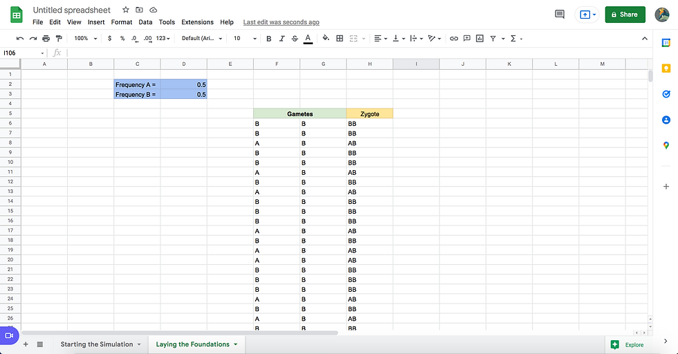
When you press enter, you will see that the two gametes in cells F6 and G6 have been linked together into a single cell to form something like AA, BB, or AB. Though this might seem like a rather pointless creation, it actually serves a very useful purpose: to simplify the rest of the formulas we want to build from this point onward. It is possible to reference the cells with the gametes, but it would be much more complicated than if we just implemented this simple summary. When it comes to spreadsheets, it pays to work smarter, not harder. Adding extra steps will usually only save you time when it comes to spreadsheets, so be sure to break up complex operations into multiple steps so that you won't find yourself writing needlessly complex formulas later on.
Go ahead and set a label for this new column of individuals--"zygote" is the appropriate scientific term here, but really all this column stands for is an individual within your population, so use whichever term best conveys that concept in your mind. Then, drag the formula down as far as you have dragged the formula for randomly generating gametes; since you didn't include dollar signs in the cell names you used in the formula earlier, the cells used will automatically shift "downward" without you needing to tweak the ranges at all! Your spreadsheet should now look something like this:
We are now only a few steps away from being able to sit back and watch the magic happen! All we need to do is find a way to sum up how many individuals of each genotype have appeared within our population. This will allow us to make the spreadsheet calculate allele frequencies and generate all kinds of interesting graphs for us!
In order to sum up all of the genotypes, we'll be paying a visit to our old friend "=IF" to put some numbers in some cells. But, first, let's set up a few more labels so that we get everything in the right place. In cell J5, write "AA"; in cell K5, write "AB"; in cell L5, write "BB." Under each of these titles, we want to put either a one or a zero in each cell. A one will signify that a certain genotype (like "AA") is the one present in that row; a zero will signify that a certain genotype is absent from the row. We will be able to use these ones and zeros to sum up how many individuals of each genotype can be found in the population!
Just like the "=IF" formula could put an "A" or a "B" in a cell, it can put a zero or a one in a cell. And, just like the "=IF" formula could compare two sets of numbers, the "=IF" formula can compare two sets of letters! Take a minute to see if you can tweak the first "=IF" formula we created, =IF(rand()<=D$2,"A","B") , to put a "1" in cell J6 if the value in cell H6 is "AA".
Done with your little experiment? Well, if you came up with the formula =IF(H6="AA",1,0), congratulations! If not, allow me to explain.
When it comes to spreadsheets, we have to put any specific sets of words or letters in quotation marks to keep the spreadsheet from getting confused. That is why the AA in the above formula has quotation marks around it, and it is also why we put quotations around A and B in the original formula. A less-than sign ("<") was not included in this formula because we want to see if the contents of cell H6 are exactly equal to "AA," not somehow less than. Finally, we simply swapped the "true" value with 1 and the "false" value with 0; this will tell the spreadsheet to put a 1 in the cell if H6 contains "AA" and a 0 in the cell if H6 contains anything else.
Go ahead and get the formula =IF(H6="AA",1,0) pasted into cell J6 if you haven't already. If a 0 or a 1 shows up, everything is working properly! While you're at it, you can get cell L6 to do the same thing for the genotype "BB" by pasting the same formula into it and changing the "AA" into "BB." Nice and simple!
We'll have to jump through a few more hoops for the last genotype, "AB," however. The way we've set up our spreadsheet so far, it is possible for the genotype to show up as either "AB" or "BA" depending on the order of the gametes. How can we get the =IF formula to make its comparisons based on two things instead of one? The answer lies with a nifty little thing called nested formulas. We actually used nested formulas a little bit earlier when we put =rand() inside our first =IF formula, but what we need to do here is a bit more complex.
You see, we need to essentially "chain" two =IF formulas together. The first will check for one of the options, like "AB," while the second will check for the other. Let's start with the first one; it will look something like =IF(H6="AB",1) . With this, we've told the spreadsheet to put a 1 in the cell if H6 contains "AB". Now, we need to add in the second =IF formula so that we can check for the alternate arrangement, "BA." We can accomplish this by setting a second =IF formula inside parenthesis where we would ordinarily put the "false" condition, like so: =IF(H6="AB",1,(IF())) . Now, we just need to use the =IF formula like we normally would, setting it to check for "BA". Try it for yourself! With any luck, you'll come up with the following: =IF(H6="AB",1,(IF(H6="BA",1,0))) . Altogether, this formula tells the spreadsheet to check cell H6 for the allele combo "AB"; if it isn't there, it will check again for "BA". If that isn't there either, it will put a 0 in the cell. That's the beauty of nested formulas! Go ahead and try it out in cell K6 now; if everything has been typed correctly, you'll see either a 0 or a 1.
Why so many parentheses?
That formula we just made has a whole bunch of parenthesis in it, and you might be wondering why all that is necessary. If you're at all familiar with the popular order for solving math equations, PEMDAS, you know that parentheses are the first thing that gets solved in any equation. Since a spreadsheet is basically just a more advanced graphing calculator, setting things off in parentheses helps keep the spreadsheet from "jumping ahead" or getting confused by extra formulas, just like they would in a graphing calculator. When you are nesting formulas, make sure to set them off in their own parentheses for precisely this reason, and don't forget to "close" any parentheses you "open" by pairing each left parenthesis ("(") with a right parenthesis (")"). That's why there are three right parentheses at the end of the formula we just made; without them, the formula wouldn't work correctly because the spreadsheet would be confused by all the "open" sets of parentheses. If you have any coding experience, this sort of thing should be familiar to you, since HTML prompts work in a very similar way.
Get all three of these formulas copied down as far as you have copied the gamete formulas, and you will have crested the last major hurdle before the big payoff! Now, all we really need to do is work some simple formulas to obtain summaries of our data.
Scroll all the way down to the point where your gamete and summary formulas stop. It should look something like this down there:

Our goal is to sum up all of the numbers in columns J, K, and L to see how many of each genotype there are. That can be accomplished with a cheeky little formula known as =SUM , which does exactly what you think it does. Simply put, it adds together all of the values in any cells you specify. I'll use my column for the number of AA individuals as an example, but you will probably need to tweak the formula I produce a little bit to fit the range of cells you wound up using.
Since I extended my formulas down 100 cells, the range of cells I want to sum up for the AA genotype stretches from J6 to J106. I would set up my =SUM formula as follows to include that range: =SUM(J6:J106) . That's all there is to the =SUM formula! Go ahead and create a cell in the J, K, and L columns that summarizes the individuals with each genotype using the =SUM formula. Your spreadsheet should look something like this when you're done:

You may notice that the labels I used for my summaries say "Surviving." This is because our next step will be to incorporate the effects of "natural selection" into our data; without it, each generation would be almost exactly the same as the last! We need to determine what percent of individuals from each genotype will survive and reproduce so that we can simulate certain traits being preferred over others. If you came up with an organism to base your spreadsheet on, think back to the traits each of these genotypes refer to; which genotype has the most advantage over its fellows? Which has the least? Regardless, the "AB" genotype will be a middle ground between the two, since we are using incomplete dominance for our little inquiry. Use those ideas to come up with a survival rate, a percentage of surviving individuals for that genotype. Unless you want to run this simulation for many generations, I would recommend not having the survival rates be too similar. Something like a 90% survival rate for the most successful genotype, a 70% survival rate for the AB genotype, and a 50% survival rate for the least successful genotype should allow the difference to be noticeable at a reasonable point in the simulation. If you don't have anything specific in mind for your population, I would recommend applying those values to the AA, AB, and BB genotypes respectively, since that is what I will be doing with my example spreadsheet.
Now that you've got your survival rates in mind, convert the percents into decimals. We will use these decimals to modify our earlier =SUM formulas. Simply tack on an asterisk ("*") to the end of each of the =SUM formulas alongside each genotype's survival rate to make the spreadsheet multiply the sum in each column by the appropriate survival rate.
Multiplying and dividing
Those of you who haven't used a graphing calculator may be confused about why an asterisk was included out of the blue. An asterisk is used to signify multiplication on graphing calculators and in spreadsheets. Division is signified by a left slash ("/").
You should end up with something like this:

Unfortunately, as is often the case with spreadsheets, this modification has caused a new issue: there are now decimals at the end of our sums! You can't have 0.7 of an individual, so we must find some way to get the spreadsheet to round these values up. Fortunately, the solution is not hard to come by; the =ROUNDUP formula will...round values up, just like you might imagine. Add this formula to the beginning of your =SUM formulas, replacing the SUM formula's equals sign, and wrap both the sum formula and its survival rate multiplier in a set of parenthesis like so: =ROUNDUP(SUM(#:#)*#) . Apply this to each of the =SUM cells and your spreadsheet will be back to lovely whole numbers again!
Rounding formulas
The formula =ROUNDUP has two cousins: =ROUND , which rounds a value either up or down depending on which "side" it's closest to, and =ROUNDDOWN , which rounds a value down.
We have now reached the second-to-last step before the grand finale: calculating the allele frequencies for the next generation. There is nothing new to learn for this step--in fact, the only formula we will use will be the simple =SUM formula!
In column J, beneath the cell that contains the number of surviving AA individuals, we want to display the number of A alleles in the population. We will use a simple equation to do this. Since each genotype contains two alleles, each AA individual has two A alleles and each AB individual has one A allele. Since we know how many AA and AB individuals there are, all we need to do is write an equation that multiplies the number of AA individuals by two and adds it to the number of AB individuals. That will look something like this in the language of spreadsheets: =2*[cell containing the number of AA individuals]+[cell containing number of AB individuals] . You can use this same formula in column K to display the number of B alleles--just make sure to swap the cell containing the number of AA individuals with the cell containing the number of BB individuals! Finally, in the L column, use the =SUM formula to sum up the number of A alleles and the number of B alleles (=SUM([cell that contains the number of A alleles],[cell that contains the number of B alleles]) to determine the total number of alleles.
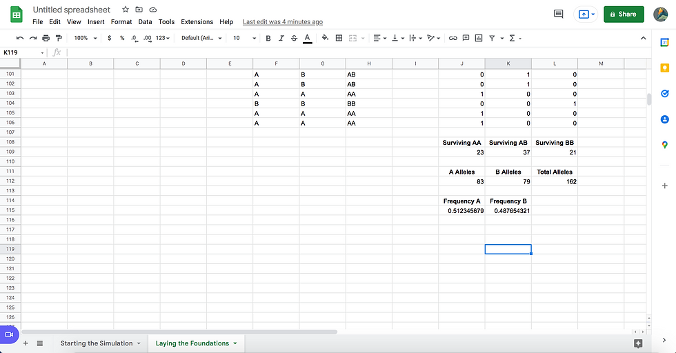
With these values in hand, all you need to do to determine the frequency of each allele is divide the number of each allele by the number of total alleles like so: =[cell containing allele number]/[cell containing the total number of alleles] ! In spare cells from the J and K columns, do this operation to find the frequency of allele A and allele B, respectively. Your spreadsheet should now look something like this:
Now, all that stands between you and watching your creation operate is a more-or-less optional step: making a graph to summarize your data. Having a visual can be really useful, but, if you don't particularly care, feel free to skip to the start of the next section where I'll show you how to get this machine you've built up and running!
For those that stayed, I will impart a brief warning: graphing is fiddly. Attempting to write out the instructions would more than likely lead to some confusion, so I have created a brief video to guide you through the process instead:
(Pardon the odd positioning of the cursor--there was an error with my video software).
Letting the Magic Happen
Now, it's finally time to watch your population change over the course of multiple different generations!
The base sheet into which we first typed all of our formulas will represent the first generation of our population. Go ahead and duplicate that initial sheet by right-clicking its tab in the bottom bar and selecting the "Duplicate" option. A new sheet that looks exactly like the first one will open up!
Instead of keeping the allele frequencies the same as for the first generation, return to your first sheet and copy the frequency of allele A. Paste this value into cell D2 in your second spreadsheet and then manually round it to two decimal places; for example, 0.475308642 would be rounded up to 0.48. With a final click of the enter key, your whole sheet will change to accommodate this new value!
Why not use the =ROUND formula?
When a spreadsheet uses the =ROUND formula to round a value with many decimal places, it will sometimes round inappropriately for frequencies. For example, you might wind up with an A allele frequency of 0.6 and a B allele frequency of 0.5--something which does not work from a mathematical standpoint! Since you need to copy and paste the frequency value anyway, it is better just to round by hand in this circumstance.
Scroll down and take a look at the graph and summary values; is a big difference between the two generations already noticeable? Keep duplicating your sheet to produce new generations, copying the frequency of the A allele from the previous generation to watch your population develop over time. Every so often, compare your most recent generation to the very first generation to see what has changed. Maybe your allele frequencies have totally shifted; maybe they have remained fairly constant, wobbling back and forth. That's the beauty of spreadsheets like these: the possibilities are endless!
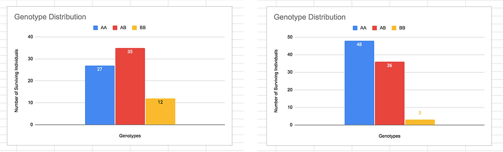
(In my spreadsheet, five generations was all it took for the BB genotype to get almost totally out-competed!)
And you aren't locked in to any one setting, either. Change your starting frequencies and see how your population develops when starting from a different place than it did during your first attempt. Change the survival rates of each genotype to see if you can drown out even the most extreme starting frequencies. And consider new lines of questioning--what if there were a third allele? What if there were more or less individuals in each generation? Now that you have the basic tools at your disposal, you can create almost anything you set your mind to with a little trial and error! And that goes for more than just population simulations--if you can dream it, you can (probably) do it with a spreadsheet, so get out and be creative!
Resources & Further Ideas
This is the very document which inspired me to create this article. The basic experiment worked out here is roughly the same as the one described in this document, but some of the spreadsheet syntax and methods from this article are outdated and difficult to use. If you want to come at this experiment from a different angle or get a sense for the background that inspired this article, feel free to check it out!
Though we covered many of the most useful formulas in this article, there are so many more to choose from and use in your future spreadsheets. This list compiled by google displays all of the formulas by name and includes links to articles that explain each one further. If you want to keep creating spreadsheets, I would recommend you check it out and learn about the other tools that might help you.
This is simply a link to the spreadsheet I used to demonstrate this experiment. If you find yourself confused about what formulas go where or how the whole thing is supposed to look, check out this spreadsheet to find what you're missing!
If you're curious as to how you might get this spreadsheet to work with three alleles instead of two, you might want to give this spreadsheet a look! This is the project I created based on the AP Biology Lab, and it is worth having a look at if you want some inspiration for a three-allele spreadsheet of your own! Just make sure you take note of the information and warnings set forward in the Introduction sheet.
Spreadsheet Idea: Spreadsheet Battleship
Have you ever heard of the popular board game, Battleship? If you have, you might want to try your hand at recreating it in a Spreadsheet! This can be as simple or complex as you like; you can learn new formulas to automate the whole process or use the simple formulas you learned in this tutorial to create a more rudimentary version. If you're looking for a fun way to play around with spreadsheets, this is a great place to start! You can even play it with friends by using the Google Sheets "share" function.
Comments